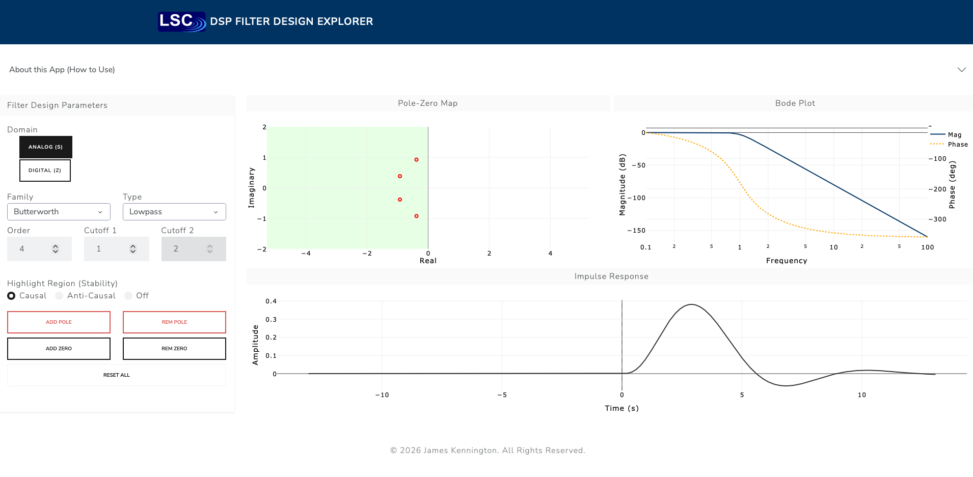
Interactive App: Digital Signal Processing Explorer
Motivation: From Equations to Intuition
Signal processing is often taught through static diagrams and theorems. We learn that “poles on the left half-plane are stable” or “zeros on the unit circle kill frequencies,” but these concepts remain abstract algebraic rules for many students.
To bridge this gap, I built the DSP Filter Design Explorer—an open-source, interactive pedagogical tool built with Python and Dash. It allows students and engineers to “play” with filter topology and see the immediate consequences in both the frequency and time domains.
Key Features
1. Unified Analog & Digital Design
The app unifies the two worlds of DSP by treating them as selectable domains with their own stability logic: * Analog (\(s\)-plane): Stability is defined by the Left Half Plane. The imaginary axis (\(j\omega\)) represents frequency. * Digital (\(z\)-plane): Stability is defined by the Unit Circle. The angle around the circle represents frequency (from DC to Nyquist).
2. Interactive Geometry
Standard textbook filters (Butterworth, Chebyshev) act as starting points, but you aren’t limited to them. You can grab any pole or zero and drag it to a new location. This allows for “What if?” exploration: What happens if I break the symmetry of this Butterworth filter? What if I move this pole dangerously close to the stability boundary?
3. Stability Visualization
A “Highlight Region” toggle visually demarcates the Causal (Stable) and Anti-Causal regions. * In Analog mode, you see the classic Left/Right plane split. * In Digital mode, you see the interior/exterior of the Unit Disk.
Interactive Learning Labs
The best way to build intuition for signal processing is to experiment. Here are five exercises you can run in the app to explore stability, causality, and symmetry.
Experiment 1: The Time-Stability Connection
Setup: Select Analog mode. Ensure the Causal region is highlighted (Green on the left). Action: Take a single pole from the stable Left Half Plane (Green) and drag it across the vertical axis into the Right Half Plane (Red). Observation: * In Green Zone: The impulse response decays forward in time (\(t > 0\)). * On the Line: The signal oscillates forever (Marginally Stable). * In Red Zone: The signal does not explode. Instead, it flips! It now decays backward in time (\(t < 0\)).
This app prioritizes Stability over Causality. Mathematically, a pole in the Right Half Plane (\(Re(s) > 0\)) corresponds to an exponential \(e^{st}\) that grows infinitely as \(t \to \infty\). To keep the energy bounded (stable), the math engine treats this pole as “Anti-Causal”—meaning the signal must decay from the future (\(t=0\)) back into the past (\(t \to -\infty\)).
Experiment 2: Zeros as “Notches”
Zeros effectively “kill” frequencies. Setup: Click “Reset”, switch to Analog, and click Add Zero. Action: Drag the blue zero directly onto the imaginary axis (the central vertical line) at a specific height (e.g., \(y=2\)). Observation: Look at the Bode Plot (Magnitude). You will see a sharp dip (a notch) descending to \(-\infty\) dB at that exact frequency.
The transfer function is a ratio: \(H(s) = \frac{\text{Zeros}}{\text{Poles}}\). If you place a zero exactly at a specific frequency \(s = j\omega\), the numerator becomes zero, and the gain drops to nothing. This is exactly how engineers design filters to remove 60Hz power line hum!
Experiment 3: The “Speed vs. Ringing” Trade-off
Setup: Select Lowpass and Order 4. Action: Toggle between the Butterworth and Chebyshev I families. Observation: * Butterworth: Poles form a wide semi-circle. The impulse response decays quickly but smoothly. * Chebyshev: Poles are squashed into an ellipse closer to the imaginary axis. The impulse response “rings” (oscillates) for much longer.
As poles move closer to the stability boundary (the imaginary axis), their “damping ratio” decreases. * Butterworth maximizes distance from the axis for a given cutoff, resulting in minimal ringing. * Chebyshev pushes poles closer to the danger zone to get a steeper frequency cutoff, but pays the price with longer time-domain ringing.
Experiment 4: Building a Stable Anti-Causal Filter
Textbooks often say “Anti-Causal filters are impossible.” That is only true for real-time hardware. In data post-processing, they are very real. Setup: Select Analog mode. Action: Drag ALL poles into the Right Half Plane. Observation: You will see a stable, bounded impulse response that exists entirely in negative time (\(t < 0\)).
This demonstrates that “Unstable” poles are only unstable if you force them to process data from the past. If you reverse your data stream (processing from end to start), these “Unstable” poles become stable! This is the core principle behind “Forward-Backward Filtering” (filtfilt), used to smooth data without shifting it in time.
Experiment 5: Perfect Symmetry (Zero-Phase)
Setup: Click “Reset”. Action: Create a symmetric “mirror” image. For every pole you place on the left (e.g., at \(-1 + 1j\)), place a matching pole on the right (\(+1 + 1j\)). Do the same for the conjugate pairs (bottom half). Observation: The Impulse Response becomes a perfectly symmetric pulse centered at \(t=0\).
You have balanced the Phase Delay. * The Left-Hand poles delay the signal (pushing energy to \(t > 0\)). * The Right-Hand poles “advance” the signal (pulling energy to \(t < 0\)). When balanced perfectly, the phase shifts cancel out, leaving a “Zero-Phase” filter. This preserves the shape of pulses in your data better than any standard causal filter can.
The Tech Stack
The application is a pure Python stack, demonstrating that you don’t need complex JavaScript frameworks to build high-performance engineering tools.
- Dash: Handles the frontend UI and client-side state management (
dcc.Store), ensuring the app scales to many concurrent users without shared-state conflicts. - Plotly: Provides the interactive graphing. The drag-and-drop functionality is powered by Plotly’s shape-editing API.
- SciPy: The calculation engine. It handles the complex polynomial algebra (
zpk2tf), frequency response (freqs/freqz), and filtering (lfilter/impulse). - Render: Hosting provider for the Dockerized application.
Handling Edge Cases
One interesting challenge was handling “Improper” transfer functions. In the analog domain, if a user adds more zeros than poles, the system acts as a differentiator with infinite bandwidth. The app detects this topological violation and displays a warning instead of crashing the solver.
Try It Yourself
You can run the app locally or use the hosted version:
pip install dsp-filter-design
dsp-fd